
Planetary Dynamos and Space Weather
How Earth's convecting liquid-iron core sustains a self-exciting geodynamo, and how solar-wind MHD reconnection drives geomagnetic storms and space weather.
Earth’s Invisible Shield—and the Swirling Iron Engine Beneath Us
Every compass needle points north, and every night at high latitudes the aurora dances across the sky, because of magnetohydrodynamics operating on a planetary scale. Without Earth’s magnetic field, the solar wind—a supersonic stream of magnetized plasma rushing out from the Sun at 400–800 km/s—would gradually strip away our upper atmosphere, much as it helped erode the atmosphere of Mars.
Where does this planetary shield come from? Not from a giant permanent bar magnet—the Earth’s interior is far hotter than the Curie temperature of iron (~770 °C), above which permanent magnetism vanishes. Instead, 2900 km beneath our feet lies the outer core: a spherical ocean of liquid iron-nickel alloy ($R_o \approx 3480\text{ km}$) churning by thermal and compositional convection as the solid inner core slowly freezes. Because liquid iron is an electrical conductor and the Earth rotates, this convective motion acts as a self-exciting geodynamo, converting kinetic and buoyancy energy into a self-sustaining magnetic field.
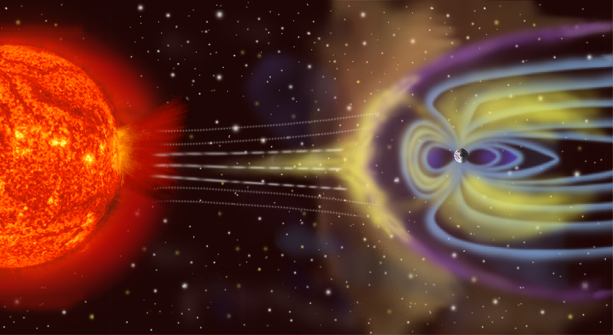
From Core Convection to Space Weather
The planetary MHD story spans two coupled domains:
- Inside the Core (Geodynamo): Buoyancy from cooling and light-element rejection at the inner-core boundary drives convective plumes twisted into helical columns by the Coriolis force. Over thousands of years, the dipole field fluctuates, drifts westward, and even flips polarity completely in geomagnetic reversals (Glatzmaier & Roberts, 1995).
- Above the Atmosphere (Space Weather): Outside Earth, the dipolar field meets the solar wind at the magnetopause ($\sim 10\,R_E$ sunward), forming a collisionless bow shock. When an interplanetary coronal mass ejection (CME) carries a southward interplanetary magnetic field ($B_z < 0$), magnetic reconnection rips open dayside field lines, dumping terawatts of energy into the magnetosphere—inducing geomagnetically induced currents (GICs) in power grids, disrupting GNSS satellites, and lighting up the aurora.
Professional Deep Dive: Dynamo Threshold, $\alpha\Omega$ Kinematics & Magnetostrophic Balance
1. The Induction Equation & Magnetic Reynolds Number
In a moving conductor of magnetic diffusivity $\eta = (\mu_0 \sigma)^{-1}$, magnetic field evolution obeys the induction equation:
$$\frac{\partial \mathbf{B}}{\partial t} = \nabla \times (\mathbf{u} \times \mathbf{B}) + \eta \nabla^2 \mathbf{B}$$Without flow ($\mathbf{u} = 0$), Earth’s core field would decay on the ohmic diffusion timescale $\tau_\eta = R_o^2 / (\pi^2 \eta) \approx 2\times 10^4\;\text{years}$—far shorter than the $3.5\;\text{Gyr}$ paleomagnetic record. Sustaining the field requires stretching and folding field lines faster than they diffuse, quantified by the magnetic Reynolds number:
$$Rm = \frac{u L}{\eta} = \mu_0 \sigma u L$$For Earth’s outer core ($u \sim 4\times 10^{-4}\;\text{m/s}$, $L \sim 2\times 10^6\;\text{m}$, $\eta \sim 1\;\text{m}^2/\text{s}$), $Rm \sim 500\text{--}1000$, safely above the dynamo threshold $Rm_{\text{crit}} \sim 40\text{--}100$.
2. The $\alpha\Omega$ Dynamo Mechanism & Cowling’s Theorem
By Cowling’s anti-dynamo theorem, a purely axisymmetric magnetic field cannot be maintained by axisymmetric flows. Nature bypasses this via 3D helical turbulence (Parker, 1955):
- $\Omega$-effect: Differential rotation shears poloidal field lines ($B_r, B_\theta$) into strong toroidal loops ($B_\phi$).
- $\alpha$-effect: Rising and sinking convective columns twisted by the Coriolis force ($2\boldsymbol{\Omega} \times \mathbf{u}$) possess non-zero kinetic helicity $\langle \mathbf{u} \cdot (\nabla \times \mathbf{u}) \rangle \neq 0$, lifting and twisting toroidal loops back into poloidal loops to close the feedback cycle.
3. Force Balances & Planetary Scaling Laws
In rapidly rotating planetary cores, inertia and viscosity are tiny compared to rotation and Lorentz forces, measured by the Ekman number $E = \frac{\nu}{\Omega L^2} \sim 10^{-15}$ and Rossby number $Ro = \frac{u}{\Omega L} \sim 10^{-6}$. The leading-order force balance is MAC (Magnetostrophic) balance:
$$2 \rho \boldsymbol{\Omega} \times \mathbf{u} \approx -\nabla p + \mathbf{J} \times \mathbf{B} + \rho' \mathbf{g}$$The strength of the Lorentz force relative to Coriolis is the Elsasser number $\Lambda = \frac{\sigma B^2}{\rho \Omega} \sim O(1)$ in Earth’s core ($B_{\text{int}} \sim 2\text{–}4\text{ mT}$). Across planets from Mercury and Ganymede to Jupiter and exoplanets, 3D geodynamo simulations (Christensen, 2010) show that internal magnetic energy density scales robustly with available convective buoyancy power $P_{\text{conv}}$ rather than rotation rate alone: $B^2 / (2\mu_0) \propto \rho^{1/3} (P_{\text{conv}}/V)^{2/3}$.
Laboratory Dynamo Experiments: Testing Planetary Magnetism on Earth
Because numerical simulations cannot simultaneously reach Earth’s extreme Ekman ($E \sim 10^{-15}$) and magnetic Prandtl ($Pm = \nu/\eta \sim 10^{-6}$) numbers, liquid-sodium laboratory dynamos provide an essential experimental bridge. Achieving $Rm > Rm_{\text{crit}} \sim 20\text{–}50$ in the laboratory requires meter-scale vessels of molten sodium ($\eta \approx 0.1\;\text{m}^2/\text{s}$) driven at $10\text{–}20\;\text{m/s}$:
- Riga Dynamo Experiment (Latvia, 1999): Led by A. Gailītis, O. Lielausis, and collaborators at IPUL (Salaspils) and HZDR, the Riga facility achieved the world’s first homogeneous self-exciting fluid dynamo in November 1999 (Gailitis et al., 2000). A single propeller drove a helical Ponomarenko-type sodium flow inside a 3 m tall cylinder, demonstrating both kinematic growth and nonlinear saturation.
- Karlsruhe Dynamo Experiment (Germany, 1999): At Forschungszentrum Karlsruhe (KIT), R. Stieglitz and U. Müller (2001) pumped liquid sodium through a 52-tube array of helical channels (a physical realization of the Roberts–Busse two-scale $\alpha^2$-dynamo), proving that small-scale helical flows generate a large-scale steady dipole field.
- VKS Dynamo Experiment (Cadarache, France, 2006): Using counter-rotating impellers in a cylindrical sodium vessel (von Kármán swirling flow), the VKS collaboration observed not only self-excitation in a strongly turbulent flow ($Re \sim 10^7$) but also spontaneous geomagnetic-like polarity reversals (Berhanu et al., 2007).
- Next-Generation Rotating & Precession Dynamos: Building on these milestones, facilities such as DRESDYN (HZDR, precession-driven 2 m sodium cylinder), UCLA SpinLab (rotating liquid-metal spherical-shell convection and magnetostrophic turbulence), and the Madison Plasma Dynamo Experiment explore rotation-dominated and plasma regimes closer to planetary cores and stars.
Key Milestones & Literature Review
- Mean-Field $\alpha\Omega$ Dynamo Theory (1955): Eugene N. Parker (1955) solved the bypass around Cowling’s anti-dynamo theorem by proposing that cyclonic convective updrafts twist toroidal magnetic flux back into poloidal loops ($\alpha$-effect), closing the self-sustaining hydromagnetic dynamo cycle.
- First 3D Polarity-Reversal Simulation (1995): Gary A. Glatzmaier and Paul H. Roberts (1995) achieved the first self-consistent 3D MHD geodynamo simulation in a rotating spherical shell, spontaneously reproducing a dipole-dominated field, westward drift, and a full geomagnetic polarity reversal.
- Universal Planetary Scaling Laws (2010): Ulrich R. Christensen (2010) analyzed over a hundred numerical dynamo runs to show that planetary and stellar field strengths obey a buoyancy-flux power law independent of viscosity and magnetic diffusivity.
- Modern Geodynamo Synthesis (2013): Paul H. Roberts and Eric M. King (2013) reviewed core energetics, magnetostrophic force balance, and the convergence between asymptotic theory, numerical simulations, and laboratory liquid-sodium dynamos.
References
- Roberts, P. H., & King, E. M. (2013). On the genesis of the Earth's magnetism. Reports on Progress in Physics, 76(9), 096801. https://doi.org/10.1088/0034-4885/76/9/096801
- Glatzmaier, G. A., & Roberts, P. H. (1995). A three-dimensional self-consistent computer simulation of a geomagnetic field reversal. Nature, 377(6546), 203–209. https://doi.org/10.1038/377203a0
- Parker, E. N. (1955). Hydromagnetic Dynamo Models. The Astrophysical Journal, 122, 293–314. https://doi.org/10.1086/146087
- Christensen, U. R. (2010). Dynamo Scaling Laws and Applications to the Planets. Space Science Reviews, 152, 565–590. https://doi.org/10.1007/s11214-009-9553-2
- Gailitis, A., Lielausis, O., Dement'ev, S., Platacis, E., Cifersons, A., Gerbeth, G., Gundrum, T., Stefani, F., Christen, M., Hänel, H., & Will, G. (2000). Detection of a Flow Induced Magnetic Field Eigenmode in the Riga Dynamo Facility. Physical Review Letters, 84(19), 4365–4368. https://doi.org/10.1103/PhysRevLett.84.4365
- Stieglitz, R., & Müller, U. (2001). Experimental demonstration of a homogeneous two-scale dynamo. Physics of Fluids, 13(3), 561–564. https://doi.org/10.1063/1.1331315
- Berhanu, M., Monchaux, R., Fauve, S., Mordant, N., Pétrélis, F., Chiffaudel, A., Daviaud, F., Dubrulle, B., Marié, L., Ravelet, F., Bourgoin, M., Odier, P., Pinton, J.-F., & Volk, R. (2007). Magnetic field reversals in an experimental turbulent dynamo. Europhysics Letters (EPL), 77(5), 59001. https://doi.org/10.1209/0295-5075/77/59001